Solving Inverse Problems with a Unified Plug-In Principle
This page organizes GLOVEX's recent and growing collection of plug-in methods for solving inverse problem in various domains with pretrained generative priors.
Estimate \(\boldsymbol{x}\) from indirect measurements \(\boldsymbol{y} \approx \mathcal A(\boldsymbol{x})\), where \(\mathcal A\) is the forward model to encode the measurement process.
Are there many of them?
Yes, everywhere in science and engineering, but phrased as reconstruction, recovery, estimation, restoration, inverse modeling, inverse design/control, conditional generation, data assimilation problems, depending on the domain.
Are they easy to solve?
No, \(\boldsymbol{x}\) is often not uniquely recoverable from \(\boldsymbol{y}\), i.e., the problem is ill-posed, so we need to use prior knowledge about \(\boldsymbol{x}\) to make the problem solvable.
Classic optimization formulation inspired by the Maximum A Posterior (MAP) principle
Here minimizing \(\ell(\boldsymbol{y},\mathcal{A}(\boldsymbol{x}))\) ensures \(\boldsymbol{y} \approx \mathcal{A}(\boldsymbol{x})\), and \(\Omega(\boldsymbol{x})\), the regularization term, encodes the prior knowledge about \(\boldsymbol{x}\) to make the problem well-posed.
How can pretrained flow-based models be used as generative priors on \(\boldsymbol{x}\)?
By flow-based models, we mean diffusion models (DMs) and flow-matching (FM) models.
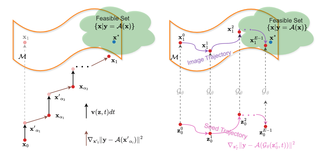
There are two families of methods, as shown above: (Left) Interleaving Methods alternate between flow generative steps and measurement-inconsistency reduction steps; (Right) Plug-in Methods directly minimize the measurement inconsistency with the generative priors plugged into the objective:
where \(\mathcal G_{\boldsymbol{\theta}}\) is the whole pretrained generation process, and the optimization is over the latent variable \(\boldsymbol{z}\). These two families of methods are contrasted in the table below (\(\widehat{\boldsymbol{x}}\) is the final estimate)
Desired property
Interleaving
Plug-in, represented by DMPlug
Manifold feasibility
\(\widehat{\boldsymbol{x}} \approx \mathcal{G}_{\boldsymbol{\theta}}(\boldsymbol{z})\) for some \(\boldsymbol{z}\)
✕
not guaranteed
✓
guaranteed, as \(\boldsymbol{x}\) reparametrized with \(\boldsymbol{x} = \mathcal{G}_{\boldsymbol{\theta}}(\boldsymbol{z})\) directly
stable estimation when \(\boldsymbol{y}\) is noisy or \(\mathcal{A}\) is imperfectly known
✕
not guaranteed and rarely tested
✓
handled via regularization and principled early-stopping rule
DMPlug
Hengkang Wang, Xu Zhang, Taihui Li, Yuxiang Wan, Tiancong Chen, Ju Sun. A Plug-in Method for Solving Inverse Problems with Diffusion Models. NeurIPS 2024. Paper.
Code.
Visual results of DMPlug
Inpainting
MeasurementReconstruction
Nonlinear deblur
MeasurementReconstruction
Super-resolution
MeasurementReconstruction
Turbulence
MeasurementReconstruction
DMPlug applied to video restoration
Hengkang Wang, Yang Liu, Huidong Liu, Chien-Chih Wang, Yanhui Guo, Hongdong Li, Bryan Wang, Ju Sun. Temporal-Consistent Video Restoration with Pre-trained Diffusion Models
. AAAI 2026. Paper.
Are foundation flow-based models more powerful as generative priors?
Generative models for domains such as images and videos are trained on internet-scale data, and hence are foundational enough to be considered as universal generators. Do these powerful generative models lead to powerful generative priors for inverse problems?
We focus on the recent flow-matching (FM) models for images, and compare foundation (FD) FM priors, domain-specific (DS) FM priors, and untrained generative priors (DIP) for Gaussian deblurring on AFHQ-Cat. Reported in our FMPlug paper.
PSNR↑
SSIM↑
LPIPS↓
DIP
27.5854
0.7179
0.3898
D-Flow (DS)
28.1389
0.7628
0.2783
D-Flow (FD)
25.0120
0.7084
0.5335
D-Flow (FD-S)
25.1453
0.6829
0.5213
FlowDPS (DS)
22.1191
0.5603
0.3850
FlowDPS (FD)
22.1404
0.5930
0.5412
FlowDPS (FD-S)
22.0538
0.5920
0.5408
Upshot: foundation flow-based priors \(\ll\) domain-specific priors, and even untrained generative priors
Isn't it surprising?
No. Power in generation and power as priors for solving IPs demand different things. Foundation flow-based models are powerful as generators in the sense that \(\mathcal G_{\boldsymbol{\theta}}(\boldsymbol{z})\) can generate virtually everything given an appropriate seed \(\boldsymbol{z}\), but they are weak when used as generative priors for inverse problems in the sense they provide weak constraints on the solution space.
FMPlug
Yuxiang Wan, Ryan Devera, Wenjie Zhang, Ju Sun. Saving Foundation Flow-Matching Priors for Inverse Problems
. ICML 2026. Paper.
Code.
Yuxiang Wan, Ryan Devera, Wenjie Zhang, Ju Sun. FMPlug: Plug-In Foundation Flow-Matching Priors for Inverse Problems. International Workshop on Computational Advances in Multi-Sensor Adaptive Processing (CAMSAP) 2025. Paper.
How to save the weak foundation flow-based priors, then?
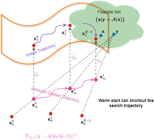
In FMPlug, we assume that additional guide samples close to the target \(\boldsymbol{x}\) are available, and propose augmenting the weak foundation flow-based prior on \(\boldsymbol{x}\) by guidance from these samples.
Instance-guided warm-start
Assume \(\boldsymbol{x}_0\) is a sample close to the target \(\boldsymbol{x}\). The ideal flow path in flow-based models is
\[
\boldsymbol{x}_t = \alpha_t \boldsymbol{x} + \beta_t \boldsymbol{z} \quad t\in[0,1],
\]
which can be approximated by
\[
\boldsymbol{x}_t \approx \alpha_t \boldsymbol{x}_0 + \beta_t \boldsymbol{z},\quad t\in[0,1].
\]
with an approximation error \(\alpha_t \|\boldsymbol{x}_0-\boldsymbol{x}\|\). Since \(\alpha_t\) is a predefined function of \(t\), we can leave \(t\) learnable to be adaptive to \(\|\boldsymbol{x}_0-\boldsymbol{x}\|\) so that \(\alpha_t \|\boldsymbol{x}_0-\boldsymbol{x}\|\) is small.
Plugging the instance-guided warm-start into the DMPlug objective yields our FMPlug framework to save foundation flow-based priors (\(\Omega\) omitted):
Here, the constraint \(\boldsymbol{z} \in S^{d-1}_{\epsilon}(0,\sqrt{d})\) ensures that the seed \(\boldsymbol{z}\) lies in a thin Gaussian shell as dictated by the concentration of measure behavior of Gaussian random vectors (we assume the standard Gaussian source distribution). For simple image restoration problems, we can often take \(\boldsymbol{x}_0 = \boldsymbol{y}\). For linear IPs, we can often take \(\boldsymbol{x}_0 = \mathcal{A}^\dagger \boldsymbol{y}\), where \(\mathcal{A}^\dagger\) is the Moore-Penrose pseudoinverse of \(\mathcal{A}\).
Visual results of FMPlug
Gaussian deblur
MeasurementReconstruction
Inpainting
MeasurementReconstruction
Motion deblur
MeasurementReconstruction
Super-resolution
MeasurementReconstruction
FMPlug extended for scientific inverse problems with few-shot guide samples
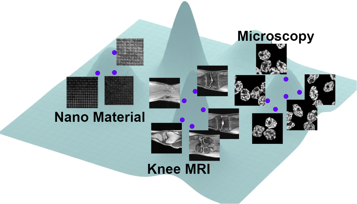
Many scientific domains are data-scarce and hence cannot afford to train domain-specific flow-based generative models. However, their adjacent domains with similar object types might already have foundation generative models, which could be repurposed for the scientific domain under consideration, e.g., generative models of natural images can be repurposed for microscopy imaging. Moreover, since scientific IPs are typically highly nonlinear, precluding guidance from \(\mathcal{A}^\dagger \boldsymbol{y}\) or \(\boldsymbol{y}\) itself as in the simple IPs above.
A scientific IP often concern data with limited variability only, allowing samples previously obtained to be used as few-shot guide samples.
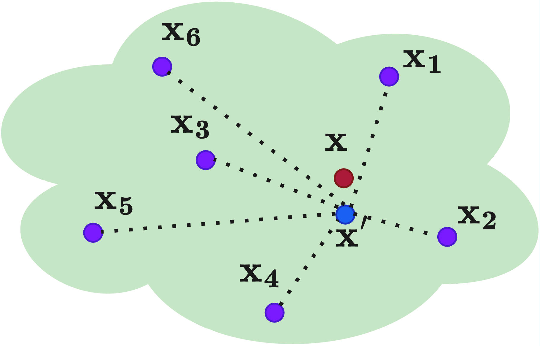
Few-shot FMPlug forms an instance-guided warm start from a linear combination of the few-shot samples, with learnable combination weights.
We consider a set of \(K\) guide samples \(\{\boldsymbol{x}_k\}_{k=1}^{K}\), some of which are close to the target \(\boldsymbol{x}\), and consider the combined guide \(\sum_{k=1}^{K}w_k \boldsymbol{x}_k\) with learnable weights \(\boldsymbol{w}\), leading to
where \(\Delta_K \doteq \{\boldsymbol{w}\in\mathbb{R}^K: w_k\geq 0, \sum_{k=1}^{K}w_k=1\}\) is the probability simplex. The simplex weights \(\boldsymbol{w}\) select and combine the most relevant few-shot instances from
\(\{\boldsymbol{x}_k\}_{k=1}^{K}\).
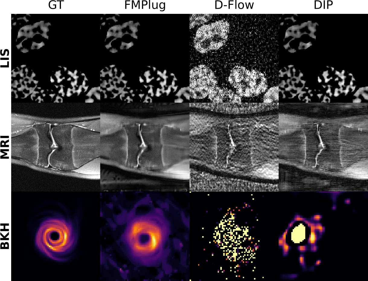
Visual results of few-shot FMPlug on scientific IPs
Comparison of few-shot FMPlug with D-Flow (another representative plug-in method) and DIP (a representative untrained generative prior method) on linear inverse scattering (LIS), compressed-sensing MRI (MRI), and black hole imaging (BKH).
GLOVEX's work on IPs with untrained generative priors
Deep image prior applied to blind deblurring with unknown kernel size
Zhong Zhuang, Taihui Li, Hengkang Wang, Ju Sun. Blind image deblurring with unknown kernel size and substantial noise. International Journal of Computer Vision, 2024. Paper.
Deep image prior applied to practical Fourier phase retrieval
Zhong Zhuang, David Yang, Felix Hofmann, David Barmherzig, Ju Sun. Practical Phase Retrieval Using Double Deep Image Priors. Electronic Imaging, 2023. Paper.
Accelerated deep image priors for simple image restoration
Taihui Li, Hengkang Wang, Zhong Zhuang, Ju Sun. Deep Random Projector: Accelerated Deep Image Prior. CVPR 2023. Paper.
Code.
Tackling overfitting issues in deep image prior
Hengkang Wang, Taihui Li, Zhong Zhuang, Tiancong Chen, Hengyue Liang, Ju Sun. Early Stopping for Deep Image Prior. TMLR 2023. Paper.
Code.